Modelado en espacio de estados

Es la representación de ecuaciones de estado de orden N en N ecuaciones diferenciales de primer orden.

El orden de las ecuaciones diferenciales es igual al número de integradores del sistema y es igual al número de variables de estado.

\[ a_n ~ y^n(t) + a_{n-1} ~ y^{n-1}(t) + ~ ... ~ + a_1 ~ \dot{y}(t) + a_0 ~ y(t) = u(t) \]

Para podemos representar las ecuación diferencia ordinaria anterior en espacio de estados, lo que haremos es defir las variables de estado \(x_1,x_2,x_3~ \cdots ~ x_n\) como:

\[\begin{split} \begin{matrix} \begin{array}{c} x_1 = y\\ x_2 = \dot y\\ x_3 = \ddot y\\ \vdots\\ x_{n-1} = y^{n-2}\\ x_n = y^{n-1} \end{array} & \left \{ \begin{array}{l} \dot{x_1} = x_2 = \dot y \\ \dot{x_2} = x_3 = \ddot y \\ \dot{x_3} = x_4 = y^{3} \\ \vdots \\ \dot x_{n-1} = x_n = y^{n-1} \\ \dot x_{n} = y_n = -\frac{a_{n-1}}{a_n} x_n - \cdots - \frac{a_{1}}{a_n} x_2 - \frac{a_{0}}{a_n} x_1 + \frac{1}{a_n} u \end{array}\right. \end{matrix} \end{split}\]

En forma matricial se puede expresar como:

\[\begin{split} \begin{aligned} \dot{\mathbf x}(t) &=\mathbf f(\mathbf x, \mathbf u) =\mathbf A \mathbf x (t) +\mathbf B \mathbf u(t) \\ \mathbf y(t) &=\mathbf g(\mathbf x, \mathbf u) =\mathbf C \mathbf x(t) +\mathbf D\mathbf u(t) \end{aligned} \end{split}\]

desarrollando las matrices para el caso particular anterior de una entrada y una salida tenemos:

\[\begin{split} \begin{bmatrix} \dot{x_1}\\\dot{x_2}\\ \vdots \\ \dot{x_n} \end{bmatrix} = \underbrace{\begin{bmatrix} 0 & 1 & 0 & \cdots & 0 \\ 0 & 0 & 1 & \cdots & 0 \\ \vdots & \vdots & \vdots & \ddots & \vdots \\ -\frac{a_{0}}{a_n} & - \frac{a_{1}}{a_n} & -\frac{a_{2}}{a_n} &\cdots & -\frac{a_{n-1}}{a_n} \end{bmatrix}}_{=\mathbf A} \begin{bmatrix} {x_1}\\{x_2}\\ \vdots \\ {x_n} \end{bmatrix} + \underbrace{\begin{bmatrix} 0 \\0\\ \vdots \\ \frac{1}{a_n} \end{bmatrix}}_{=\mathbf B}~ u \end{split}\]

\[\begin{split} y= \underbrace{\begin{bmatrix} 1 & 0 & \cdots & 0 \end{bmatrix}}_{ =\mathbf C} \begin{bmatrix} {x_1}\\{x_2}\\ \vdots \\ {x_n} \end{bmatrix} + \underbrace{\begin{bmatrix}0\end{bmatrix}}_{= D} ~u \end{split}\]

Ejemplo de sistema electromecánico: motor eléctrico

Desarrollo de las ecuaciones

Del ejemplo anterior reescribimos las ecuaciones que describen la dinámica del motor eléctrico, de forma conveniente (en ambos casos la derivada de mayor orden a la izquierda del signo igual):

\[\begin{split} \left\{\begin{array}{c} \frac{di_a(t)}{dt} = \frac{1}{L_a} e_a(t) -\frac{ R_a}{L_a} i_a(t) - \frac{K_b}{L_a} \frac{d\theta_m(t)}{dt} \\ \frac{d^2\theta_m(t)}{dt^2} = \frac{K_t}{J_m} i_a(t) - \frac{D_m}{J_m}\frac{d\theta_m(t)}{dt} - \frac{1}{J_m} T_r(t) \end{array}\right. \end{split}\]

propondremos como variables de estados (VE) a \(i_a(t)\),\(\frac{d\theta_m(t)}{dt}\) y \(\theta_m(t)\) por lo que,

\[\begin{split} \begin{matrix} u(t) = e_a(t) &\mbox{y}& w(t)= T_r(t)\\ x_1 = i_a &\Longrightarrow & \dot{x_1}=\frac{di_a}{dt} \\ x_2 = \frac{d\theta_m(t)}{dt} &\Longrightarrow & \dot{x_2}=\frac{d^2\theta_m}{dt^2}\\ x_3 = \theta_m &\Longrightarrow & \dot{x_3}=\frac{d\theta_m}{dt} = x_2 \end{matrix} \end{split}\]

reemplazamos el cambio de variables:

\[\begin{split} \left\{\begin{array}{c} \dot{x_1} = \frac{1}{L_a} u(t) -\frac{ R_a}{L_a} x_1(t) - \frac{K_b}{L_a} x_2(t) \\ \dot{x_2} = \frac{K_t}{J_m} x_1(t) - \frac{D_m}{J_m} x_2(t) - \frac{1}{J_m} w(t)\\ \dot{x_3} = x_2 \end{array}\right. \end{split}\]

Finalmente en forma matricial tenemos que:

\[\begin{split} \begin{bmatrix} \dot{x_1}\\\dot{x_2} \\ \dot{x_3} \end{bmatrix} = ~ \underbrace{\begin{bmatrix} -\frac{ R_a}{L_a} & - \frac{K_b}{L_a} & 0\\ \frac{K_t}{J_m} & - \frac{D_m}{J_m} & 0\\ 0 & 1 & 0 \end{bmatrix}}_{=~A} ~ \begin{bmatrix} {x_1}\\{x_2}\\ {x_3} \end{bmatrix} + \underbrace{\begin{bmatrix} \frac{1}{L_a}\\0 \\0\end{bmatrix} }_{=~B} u + ~ \underbrace{\begin{bmatrix} 0\\- \frac{1}{J_m} \\0\end{bmatrix} }_{=~B_1} w\\ y = ~ \underbrace{\begin{bmatrix} 0 & 0 & 1\end{bmatrix}}_{=~C} \begin{bmatrix} {x_1}\\{x_2}\\ {x_3} \end{bmatrix} + ~ \underbrace{\begin{bmatrix} 0 \end{bmatrix} }_{=~D} u \end{split}\]

Simulación

Show code cell content Hide code cell content

import control as ctrl
import matplotlib.pyplot as plt
import numpy as np

Definimos los parámetros del sistema

Jm = 3.2284E-6
Dm = 3.5077E-6
Kb = 0.0274
Kt = 0.0274
Ra = 4
La = 2.75E-6

Con los parámetros del sistema definimos las matrices de estados

A = [[-Ra/La,-Kb/La,0],[Kt/Jm,-Dm/Jm,0],[0,1,0]]
B = [[1/La],[0],[0]]
C = [0,0,1]
D = 0

Notar que cada matriz es una lista. Esta lista contiene listas que representan cada fila de la matriz.

En caso de ser una matriz con una sola fila, la matriz de representa como una lista de float o int números en general.

Ahora vamos a definir el sistema en espacio de estados usando el paquete de control e python.

motor_ss=ctrl.ss(A,B,C,D)
motor_ss

\[\begin{split} \left(\begin{array}{rllrllrll|rll} -1.&\hspace{-1em}45&\hspace{-1em}\cdot10^{6}&-9.&\hspace{-1em}96&\hspace{-1em}\cdot10^{3}&0\phantom{.}&\hspace{-1em}&\hspace{-1em}\phantom{\cdot}&3.&\hspace{-1em}64&\hspace{-1em}\cdot10^{5}\\ 8.&\hspace{-1em}49&\hspace{-1em}\cdot10^{3}&-1.&\hspace{-1em}09&\hspace{-1em}\phantom{\cdot}&0\phantom{.}&\hspace{-1em}&\hspace{-1em}\phantom{\cdot}&0\phantom{.}&\hspace{-1em}&\hspace{-1em}\phantom{\cdot}\\ 0\phantom{.}&\hspace{-1em}&\hspace{-1em}\phantom{\cdot}&1\phantom{.}&\hspace{-1em}&\hspace{-1em}\phantom{\cdot}&0\phantom{.}&\hspace{-1em}&\hspace{-1em}\phantom{\cdot}&0\phantom{.}&\hspace{-1em}&\hspace{-1em}\phantom{\cdot}\\ \hline 0\phantom{.}&\hspace{-1em}&\hspace{-1em}\phantom{\cdot}&0\phantom{.}&\hspace{-1em}&\hspace{-1em}\phantom{\cdot}&1\phantom{.}&\hspace{-1em}&\hspace{-1em}\phantom{\cdot}&0\phantom{.}&\hspace{-1em}&\hspace{-1em}\phantom{\cdot}\\ \end{array}\right) \end{split}\]

Vamos a evaluar la respuesta del sistema frente a un cambio escalón en la tension de alimentación. Para esto primero vamos a definir un vector t donde nos interesa obtener los valores de la salida. Esto lo haremos usando la función linspace de numpy.

t=np.linspace(0,0.1,100)

El función step_response del paquete de control de python nos devolverá dos vectores: uno con los tiempo donde calculó las salidas y otro con las salidas.

t,y=ctrl.step_response(motor_ss,T=t)

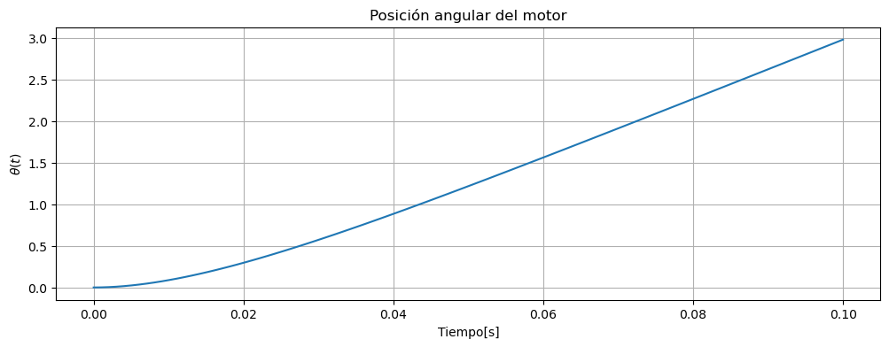
Una vez que tenemos la salida (para este caso es una sola), podemos graficarla:

Show code cell source Hide code cell source

fig, ax = plt.subplots(figsize=(12,4))
ax.plot(t,y)
ax.set_title('Posición angular del motor')
ax.set_xlabel('Tiempo[s]')
ax.set_ylabel(r'$\theta(t)$')
ax.grid()

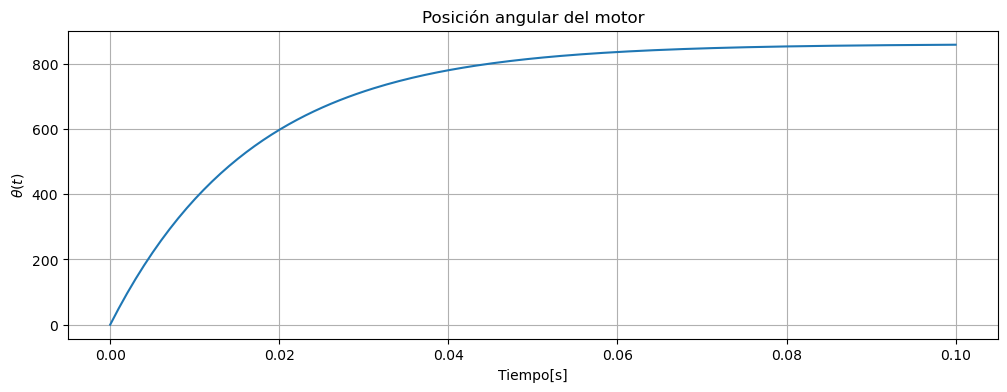
Ahora supongamos que deseamos medir velocidad angular del motor, es decir la variable de estado \(x_2\), entonces podemos definir la matriz \(C\) de la siguiente manera:

\[\begin{split}\mathbf C = \begin{bmatrix} 0 & 1 & 0\\ \end{bmatrix}\end{split}\]

y graficamos simulamos:

C=[0,1,0]
motor_vel_ss=ctrl.ss(A,B,C,D)
t=np.linspace(0,0.1,200)
t,y=ctrl.step_response(24*motor_vel_ss,T=t)

Show code cell source Hide code cell source

fig, ax = plt.subplots(figsize=(12,4))
ax.plot(t,y, label=r'$\theta$')
ax.set_title('Posición angular del motor')
ax.set_xlabel('Tiempo[s]')
ax.set_ylabel(r'$\theta(t)$')
ax.grid()

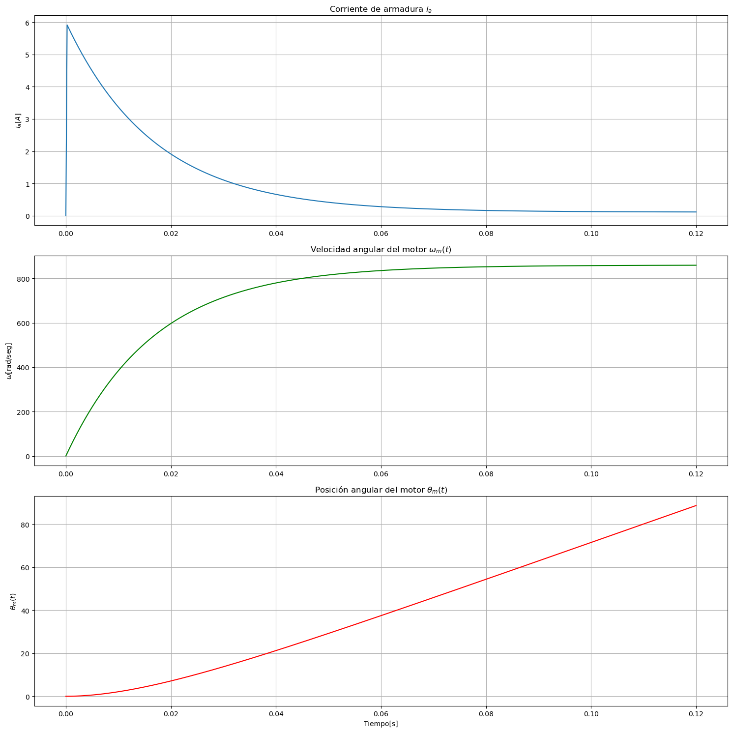
En los casos anteriores, el sistema es SISO, es decir 1 entrada y 1 salida, supongamos ahora que deseamos medir todas las variables de estado \(\theta_m(t)\) (la posición angular), \(\omega_m (t)= \frac{d\theta_m(t)}{dt}\) (la velocidad angular) y \(i_a(t)\) (la corriente de armadura), para lo que definiremos nuevamente la matriz de medición \(C\) y graficaremos las variables de estado para una entrada del tipo escalón de \(1 ~[Volt]\):

C=[[1,0,0],[0,1,0],[0,0,1]]
D=[[0],[0],[0]]
motor_ss=ctrl.ss(A,B,C,D)
motor_ss

\[\begin{split} \left(\begin{array}{rllrllrll|rll} -1.&\hspace{-1em}45&\hspace{-1em}\cdot10^{6}&-9.&\hspace{-1em}96&\hspace{-1em}\cdot10^{3}&0\phantom{.}&\hspace{-1em}&\hspace{-1em}\phantom{\cdot}&3.&\hspace{-1em}64&\hspace{-1em}\cdot10^{5}\\ 8.&\hspace{-1em}49&\hspace{-1em}\cdot10^{3}&-1.&\hspace{-1em}09&\hspace{-1em}\phantom{\cdot}&0\phantom{.}&\hspace{-1em}&\hspace{-1em}\phantom{\cdot}&0\phantom{.}&\hspace{-1em}&\hspace{-1em}\phantom{\cdot}\\ 0\phantom{.}&\hspace{-1em}&\hspace{-1em}\phantom{\cdot}&1\phantom{.}&\hspace{-1em}&\hspace{-1em}\phantom{\cdot}&0\phantom{.}&\hspace{-1em}&\hspace{-1em}\phantom{\cdot}&0\phantom{.}&\hspace{-1em}&\hspace{-1em}\phantom{\cdot}\\ \hline 1\phantom{.}&\hspace{-1em}&\hspace{-1em}\phantom{\cdot}&0\phantom{.}&\hspace{-1em}&\hspace{-1em}\phantom{\cdot}&0\phantom{.}&\hspace{-1em}&\hspace{-1em}\phantom{\cdot}&0\phantom{.}&\hspace{-1em}&\hspace{-1em}\phantom{\cdot}\\ 0\phantom{.}&\hspace{-1em}&\hspace{-1em}\phantom{\cdot}&1\phantom{.}&\hspace{-1em}&\hspace{-1em}\phantom{\cdot}&0\phantom{.}&\hspace{-1em}&\hspace{-1em}\phantom{\cdot}&0\phantom{.}&\hspace{-1em}&\hspace{-1em}\phantom{\cdot}\\ 0\phantom{.}&\hspace{-1em}&\hspace{-1em}\phantom{\cdot}&0\phantom{.}&\hspace{-1em}&\hspace{-1em}\phantom{\cdot}&1\phantom{.}&\hspace{-1em}&\hspace{-1em}\phantom{\cdot}&0\phantom{.}&\hspace{-1em}&\hspace{-1em}\phantom{\cdot}\\ \end{array}\right) \end{split}\]

Ahora podemos simular la respuesta al escalón

t=np.linspace(0,0.12,500)
t,y=ctrl.step_response(24*motor_ss,T=t)

Show code cell source Hide code cell source

fig, axes = plt.subplots(3, 1, figsize=(15, 15))

axes[0].plot(t,y[0,:].T)
axes[0].grid()
axes[0].set_title(r"Corriente de armadura $i_a$")
axes[0].set_ylabel(r'$i_a[A]$')

axes[1].plot(t,y[1,:].T, 'g');
axes[1].grid()
axes[1].set_title(r"Velocidad angular del motor $\omega_m (t)$")
axes[1].set_ylabel(r'$\omega$[rad/seg]')

axes[2].plot(t,y[2,:].T, 'r', label="y = x")
axes[2].grid()
axes[2].set_title( r"Posición angular del motor $\theta_m(t)$")
axes[2].set_xlabel('Tiempo[s]')
axes[2].set_ylabel(r'$\theta_m(t)$');

fig.tight_layout()